Getting a Grasp on Data Science: David Donoho’s Six-Part Definition

The discipline of data science is notoriously difficult to define, and yet it is perhaps not impossible. I am currently working to gear more of my thought and instruction around Stanford statistician David Donoho’s definition of Greater Data Science (GDS). Here I’ll provide a brief summary of three key contributions of Donoho’s argument, ending with his six-part definition of the discipline.

First, Donoho appropriately connects the current expansive discipline of Data Science to its roots in 50+ years of work by statisticians, beginning with John Tukey in the 1960s. On Donoho’s telling, contemporary Data Science should understand itself not in opposition to the discipline of statistics but as an outgrowth and extension of the long tradition of statistics. More than historical recognition, this extends to appreciating the contemporary relevance of both traditional statistical analysis and predictive modeling with machine learning. Just as traditional statisticians must acknowledge and embrace the importance and relevance of contemporary machine learning methods, “cutting edge” data scientists must appropriately recognize the continued role and relevance of traditional statistical analysis.

Second, Donoho helpfully identifies the Common Task Framework methodology that undergirds the successes of contemporary predictive modeling. This methodology includes (a) a publicly available training dataset, (b) a competitive multi-party approach to predictive modeling, and (c) a scoring referee or system for evaluating the competing models against a test dataset unavailable to the competitors. He cites the Netflix Challenge as a famous example of this approach.

Third, and most importantly, Donoho builds on the work of John Chambers and Bill Cleveland to outline a definition of Greater Data Science (GDS), which includes the following six sub-fields:

  1. Data Exploration and Preparation
  2. Data Representation and Transformation
  3. Computing with Data
  4. Data Modeling
  5. Data Visualization and Presentation
  6. Science about Data Science

This definition is so apt that it seems common sense to those who practice in the field. But the complexity of the work involved in data science has meant that reaching the clarity offered by this definition has not been easy. Not content simply to define, Donoho devotes the remainder of his piece to discussing and illustrating some of the key practices included under each sub-field. I will number each sub-field as he does, using GDS for Greater Data Science.

GDS1: Data Exploration and Preparation. Frequently requiring upwards of 80% of the work involved in data science, this sub-field is too often neglected in the teaching of data science and merits greater attention in the future. It includes the many steps of curating data, dealing with anomalies, and pulling into the shape needed for analysis.

GDS2: Data Representation and Transformation. This includes the problem of data storage and requires that a data science be fluent in current database technologies. As of 2021 that includes SQL and NoSQL databases, distributed (cloud) systems, etc.

GDS3: Computing with Data. This includes necessary knowledge of languages like Python or R and related current software used in preparation, analysis, and modeling, as well as understanding of the workflows used to in the development of an analytical process. 

GDS4: Data Visualization and Presentation. This sub-field addresses the importance of visual analysis methods, from standard plots used in Exploratory Data Analysis (EDA) to advanced charts used to crystalize understanding of specific important features to interactive data dashboards.

GDS5: Data Modeling. This sub-field should rightfully include both traditional statistical approaches and contemporary predictive modeling with machine learning.

GDS6: Science about Data Science. Key to making data science a true science, science of data science investigates the real-world work of data scientists “in the wild” and contributes to the documentation, description, analysis, and evaluation of those real-world practices, with the express aim of discerning the more fruitful practices that show merit for leading the discipline of data science forward to greater promise and productivity.

Given the sheer complexity of data science and the astounding speed of its ongoing development, it is difficult to overstate the value of Donoho’s six-part definition of the discipline. For myself, I will be contemplating and engaging the implications of this definition for months and years to come.

Allow me simply to recommend Donoho’s article as a read of incredible value, and recommend his helpful discussions of these six sub-fields as a beginning point for others as we work together to take the discipline forward.
 

Featured

Leveraging the narrative arc to inspire data-driven action

Great visual analytics involves a sequence of steps which may be understood as both a science and an art. That sequence includes:

  1. Understanding the business objectives. These drive and guide the analysis and provide it point and purpose.
  2. Spending the time required to understand the data inside and out. (Exploratory analysis.)
  3. Identifying and curating the most important insights, to prepare for explanatory analysis.
  4. Refining the design for clear, effective, and efficient communication, reducing clutter and highlighting key data points.
  5. Providing visual hierarchy, to draw attention to first things first, second things second, and so on.
  6. Structuring the report to provide the right mix of breadth and depth — breadth so that the stakeholders can see the big picture, and depth so that they can’t miss what’s most important. 
  7. When the occasion calls, leveraging elements of a good narrative, to lead the audience along a progression of steps from attention to recognition to engagement and finally to action.

Each of these steps merits its own extended discussion. In this post, I’d like to draw attention to the seventh step: leveraging elements of good narrative to lead the audience to action.

To my knowledge, no one has discussed this more effectively than Cole Nussbaumer Knaflic. Her book, Storytelling with Data, is the leading book on the topic, hitting many of the preceding steps, and then driving on to leverage the power of narrative in the presentation of the story.

Among the narrative elements she discusses are:

  • Establishing the setting, as a reminder of what we’re doing here and the shared goals we have.
  • Highlighting the problem as a tension between current obstacles and desired outcomes.
  • Viewing your audience as protagonists, whose actions will drive the story forward.
  • Taking a role in the story yourself, recommending possible courses of action, provoking your participants to engagement and leading toward resolution — i.e., data-driven action.

Her irrefutable point: You may have the best, most insightful, most beautifully designed analysis. But if you fail to effectively communicate that analysis, its sum total value is exactly ZERO. For at the end of the day, the sole point and purpose of analysis is to inform and generate action.

This is where Knaflic’s work is so valuable. If you’re short on time to read a book, Knaflic has presented this seventh point in the form of an entertaining and informative short video. Indeed, in this video she takes the discussion a step further to discuss the transformative power of the narrative arc:

  • Plot
  • Rising Action
  • Climax / Tension
  • Falling Action
  • Resolution / Ending

Only 15 minutes in length, her presentation is work of art. 

Properly received, her presentation should provoke you, as a data professional, to put the lesson into practice. May your future presentations be more focused, more meaningful, and much more effective at inspiring data-driven action.

Getting Started with Tableau Desktop

If you’re fairly new to Tableau, chances are you’ll find Tableau’s repository of free training videos (free with registration) to be very helpful. Indeed, there’s enough there to help you go from zero to serious just about as fast as you dare to do it. The tutorials are really pretty great.

BUT their organization scheme needs a little help.

Here’s a helpful list of the best, most useful videos to get started with. Once you’ve worked through those, check out my page with a more extensive organized index including Tableau’s more in-depth training videos.

Tableau Fundamentals

The following seven videos will get you up and running quickly.

From the Getting Started section

  1. Getting Started (25 min)
    A little lengthy, but does a great job of giving an overview of what’s possible in Tableau.
  2. The Tableau Interface (4 min)

From the Connecting to Data section

  1. Getting Started with Data (6 min) 
  2. Managing Extracts (4 min)

From the Visual Analytics section

  1. Getting Started with Visual Analytics (6 min)

From the Why is Tableau Doing That? section

  1. Understanding Pill Types (5 min) 
  2. Measure Names and Measure Values (5 min)

From this point forward, the best path depends on your needs. 

Check out my page with a more extensive organized index including Tableau’s more in-depth training videos.

Setting up an AWS Cloud Database to Support Student Projects — AWS Educate

If you’re an educator (or student) interested in leveraging Amazon Web Services through AWS Educate to host a cloud database that allows student connections — this post is for you. In what follows, I’ll document the process to:

  • Configure and create a relational database instance from the AWS Management Console.
  • Set a security profile that will allow students to read and write to the database remotely — such as from a database client, from a program they’ve written, from a Jupyter Notebook, etc.
  • I’ll illustrate the process by creating a PostgreSQL database instance. Then I’ll provide illustrative code snippets for interacting with the database using Python.

The resulting database will be friendly for student projects that include database interactions such as querying, reading, and writing.

I’m going to assume that you’ve already created your Amazon Educate Account and are logged into your AWS Console. Thus, we’ll begin by creating a relational database.


Creating a Relational Database in the AWS Console

Once you have logged into your AWS Console, these are the steps to set up a relational database.

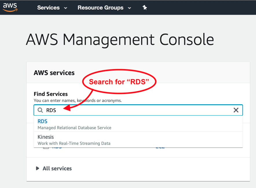
  1. Use the search field under “Find Services” to search for “RDS.” You should see RDS: Managed Relational Database Service appear in the results. Select and navigate to the RDS page.Search for RDS in AWS Console
  2. Once you’ve arrived at the Amazon RDS page, select Databases in the left-hand sidebar, and then Create Database.RDS Create Database
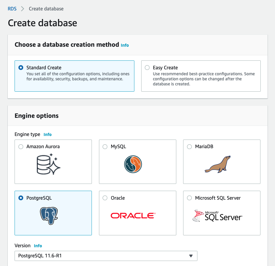
  3. From the Create Database page, select your desired options for creation method and configuration. You are free to choose differently, of course, but I have chosen these options:
    • Standard Create — This will allow me to optimize the resources my database will use.
    • PostgreSQL — A favored option among data science types. But choose what’s best for you!

      Choose creation method and database engine.
      Choose your desired creation method and database engine.

  4. Select your desired Template (the labels here may depend on the engine you choose) according to your needed system resources and the size of your budget. I currently have access to the free tier, which I’ll use now. If that were not available, Dev/Test is the next least resource-intensive option I currently have.

    Choose the template according to your needed resources
    Choose the template according to your needed resources.

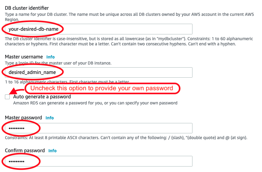
  5. If you desire, edit the database name (identifier), master username, and password.Provide desired names and password
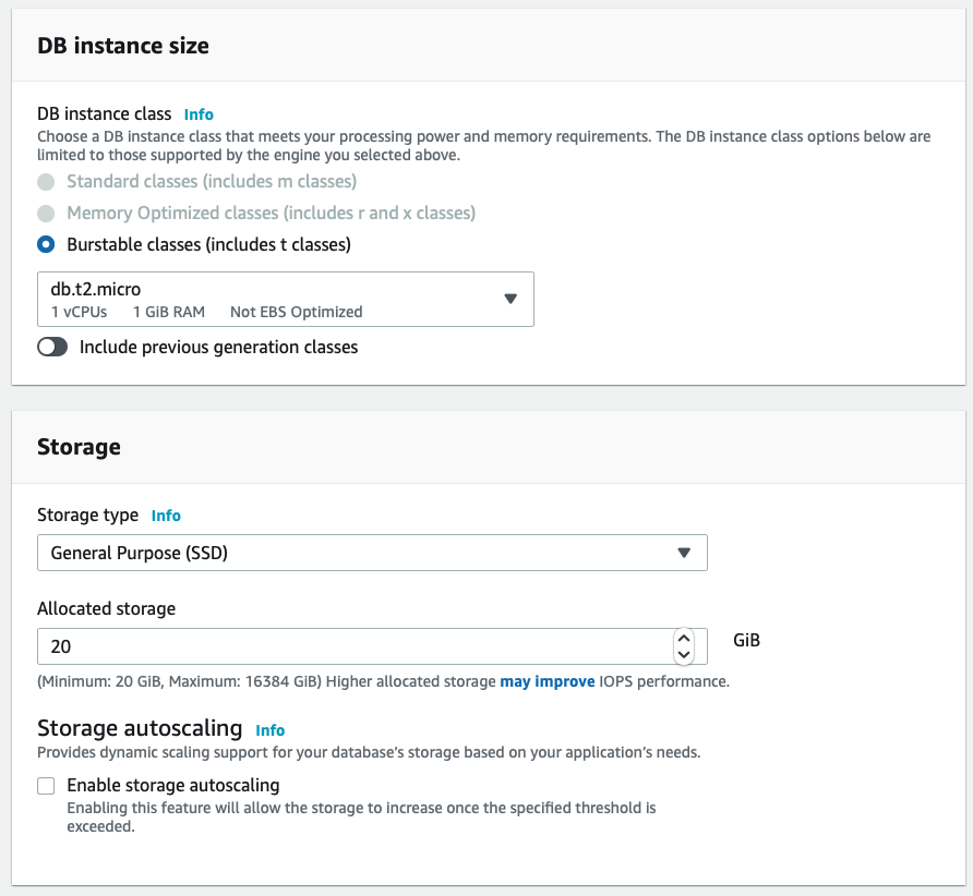
  6. Choose the DB instance size and storage (if relevant) that suits your needs and budget. I’ve chosen the least resource-intensive options, as these will be plenty for my intended use: basic CRUD operations performed by my students.

    Choose instance size and storage
    Choose instance size and storage according to the resources you need.

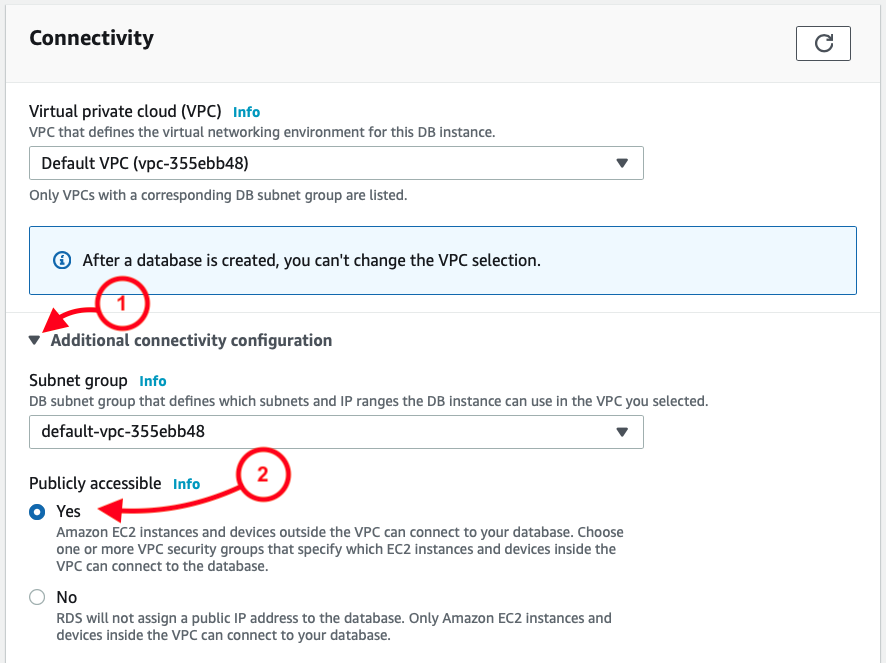
  7. Under Connectivity, select “Additional connectivity configuration” and then “Yes” under Publicly accessible.Connectivity choose publicly accessible
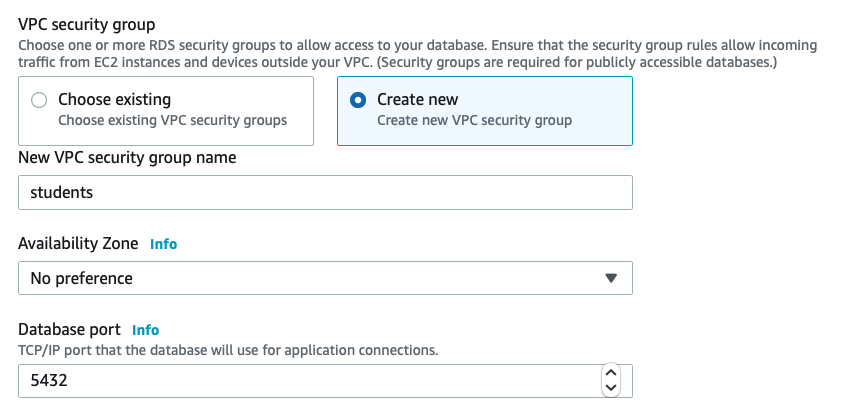
  8. You’ll be given the option to create a new security group. You can keep the default, or create a new group. I’ve created one named “students.” You’ll also see the database port settings.Security group settings
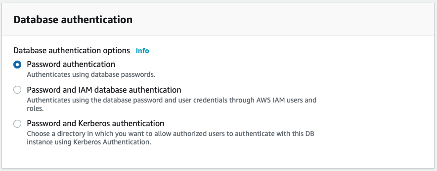
  9. Depending on your selected database engine, you may (or may not) be given the option to choose Database authentication. With the PostgreSQL database I’ve chosen, I have these options, and I’ll choose Password authentication.Database authentication options
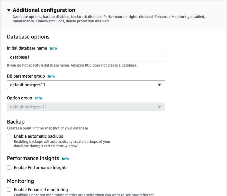
  10. Depending on your selected database engine, you may (or may not) be given Additional configuration options. If you’re unsure about these options, click the handy Info link to read more about them. I’ve deselected automatic backups in order to conserve resources.Additional configuration options
  11. If all looks good, click Create database!Click Create
  12. After clicking create, you may be given a message to go back and adjust a configuration option. If so, go back and do that. If all went well, you’ll be taken to a confirmation page. Here’s what mine looked like:Creating Database Confirmation
  13. Notice that you can click to View credential details — a handy way to get the login information and save it for future reference!


Congratulations! You’ve created your database!

Now we need to set a security rule to allow interactions with the database.


Allowing Inbound Traffic

In these next few steps, we’ll set a connection security rule to allow inbound traffic to interact with the database.

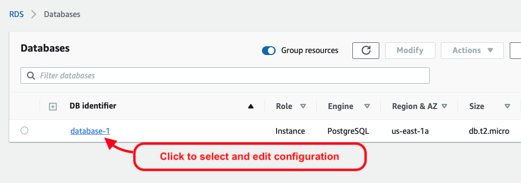
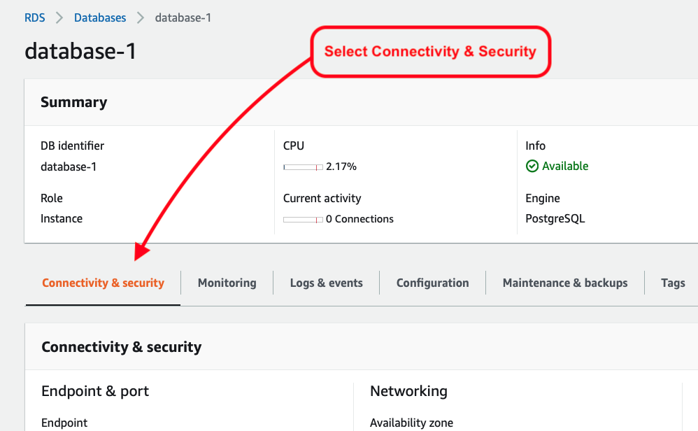
  1. Beginning at the RDS > Database page, click the database identifier.
    13_Click_to_Configure
  2. Select the Connectivity & security tab.13b_Select_Connectivity_Security
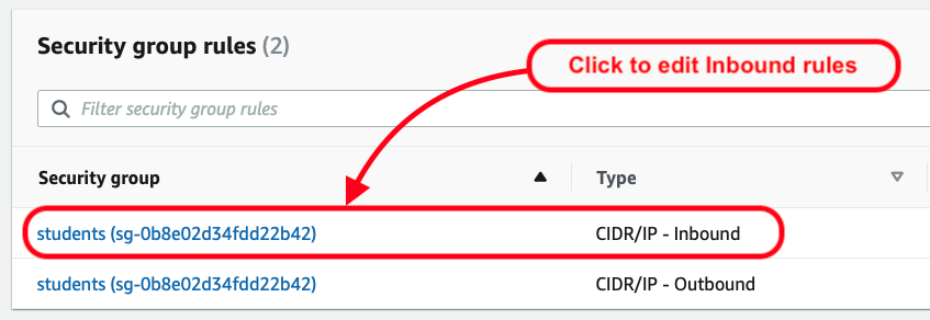
  3. Scroll down the page to Security group rules, and click to edit the Inbound rules.13a_Click_Edit_Inbound_Rules
  4. If necessary, select Actions, and Edit inbound rules.13b_Edit_Inbound_Rules
  5. There should be an initial rule begun for you. Notice that the Type and Port range are already set to match your database settings. Now we need to allow a range of IP addresses. Configure this according to your needs. In my case, I’ll be working with online students. And since the database will not contain sensitive data, I’ll simply pull down the box under Source and select “Anywhere,” to allow traffic from any IP address.14_Inbound_Rule_AnywhereOnce that’s been selected, I then see the result as two rules, allowing a full range of IP address options:
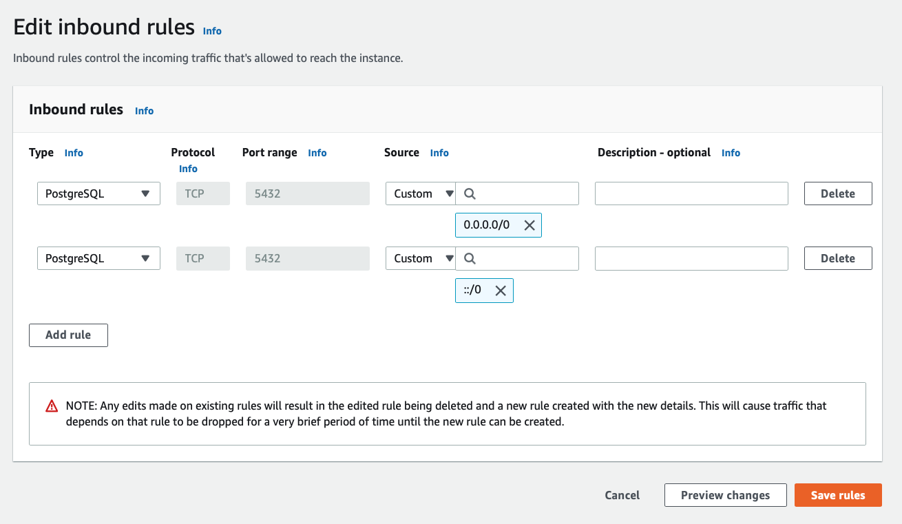
    15_Inbound_Rules
  6. Click Save rules!


Connecting to the Database

After creating the database, you can connect to the database using an application or database management package. You’ll simply need a few key items of information. These were supplied when you first created the database. The items include:

  • Endpoint (aka host or hostname)
  • Port
  • DB name
  • Master username
  • Password

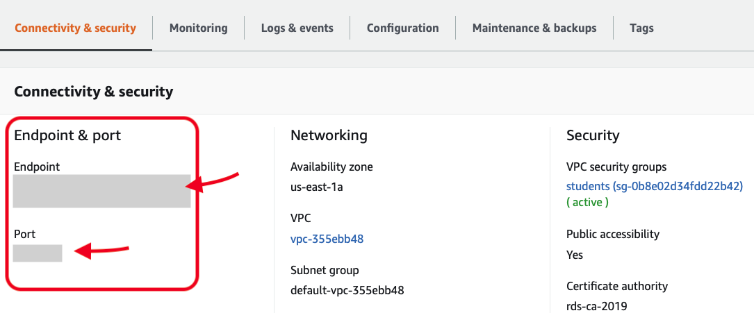
If you need to recover these later, you can do so by selecting the database from the RDS database list, and then looking under the two tabs: Connectivity & security, and Configuration.

The Endpoint (aka host or hostname) and Port can be found under the database Connectivity & Security details:

AWS database connectivity page


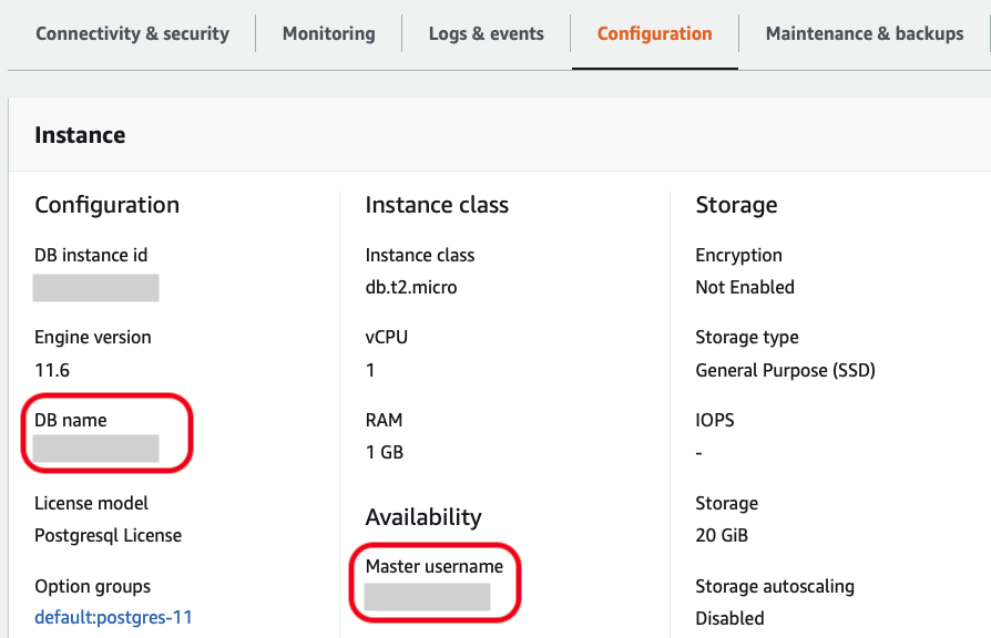
The DB name and Master username can be found under the Configuration tab:

AWS database configuration page


As for the user password, you will hopefully have recorded or remembered it!

Those provide the essential credentials you’ll need to connect to the database.

In the next section, I’ll illustrate using these credentials to connect to the database, create a table, insert records, and query the table using Python.


Interacting with the Database Using Python

Python provides modules for connecting to any number of database engines. Since I selected a PostgreSQL engine, I’ll be using the psycopg2 module to interact with it. (For a MySQL database, you can use pymysql. And so on …)

If the module is not currently installed on your system, you’ll need to install it. In Python, this may be done easily using pip or conda:

Once the module is installed, you’ll simply import it to use it in your Python application or Jupyter notebook:

import psycopg2


Next we’ll establish the connection, using the psycopg2.connect() method, and providing the database information and login credentials, such as follows:

Establish database connection using psycopg2.connect()

Then you can use lines such as follows to interact with it. (See the psycopg2 docs for guidance.)

# Start the cursor to enable SQL operations

cur = conn.cursor()

# Create a table
cur.execute("CREATE TABLE test1 (id serial PRIMARY KEY, num integer, data varchar);")

# Insert a record
cur.execute("INSERT INTO test1 (num, data) VALUES (%s, %s)", 
(101, "abcdefg"))

# Query the table
cur.execute("SELECT * FROM test1;")

# Output the query results
cur.fetchall()

# Commit the changes
conn.commit()

# Close the connection
conn.close()


In Closing

That’s it! Your database is ready to roll.

AWS Educate provides a fantastic opportunity to equip students with cloud resources. In fact, it’s worth pointing out that both educators and students can follow these steps. If a professor should want students to create their own cloud databases for their projects, the above steps will serve them just as well.

I hope this resource proves helpful. Please comment with feedback, suggestions, and recommendations!

Two Cheers for Penguins Data!!

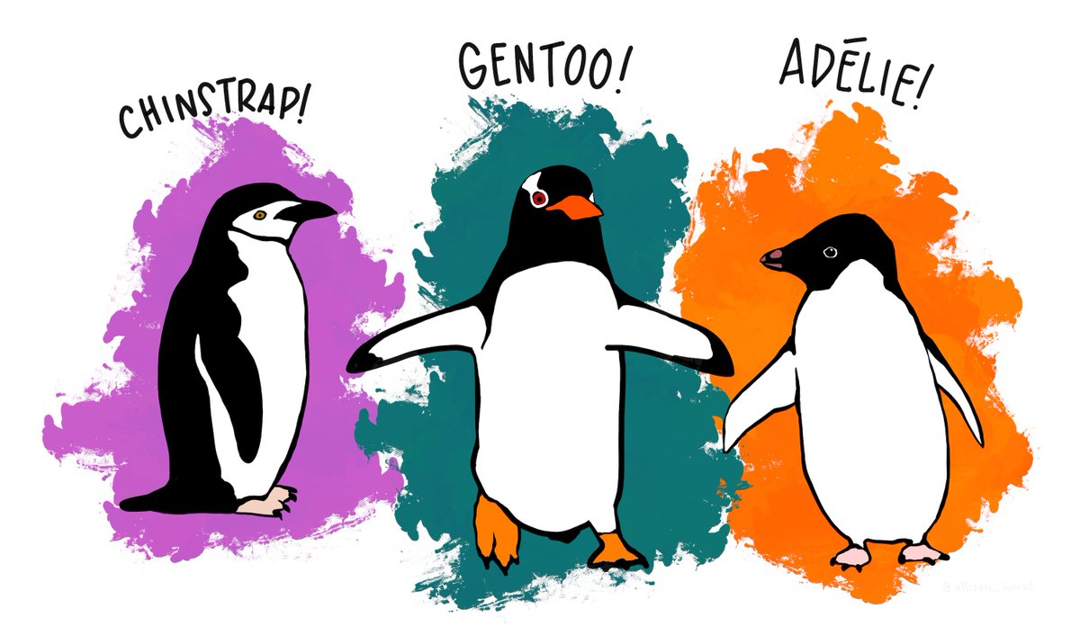
I’m excited about this penguins data set which has just been made publicly available. This will be much more fun for student projects than the old standard iris data set.

Penguins cartoon to illustrate the penguins data set

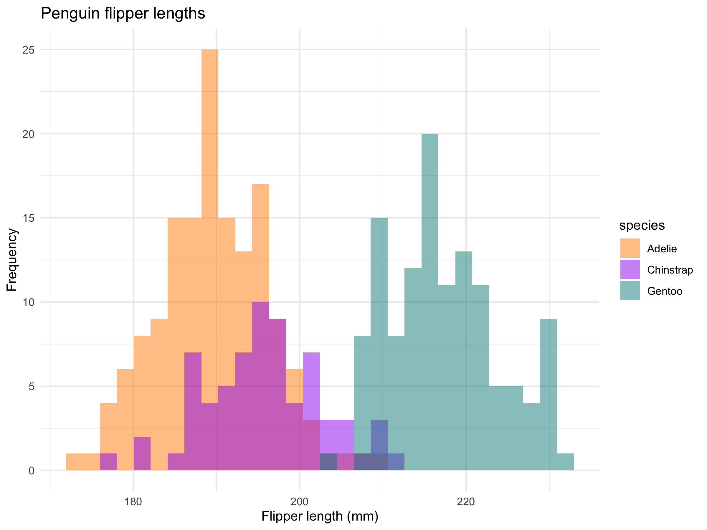
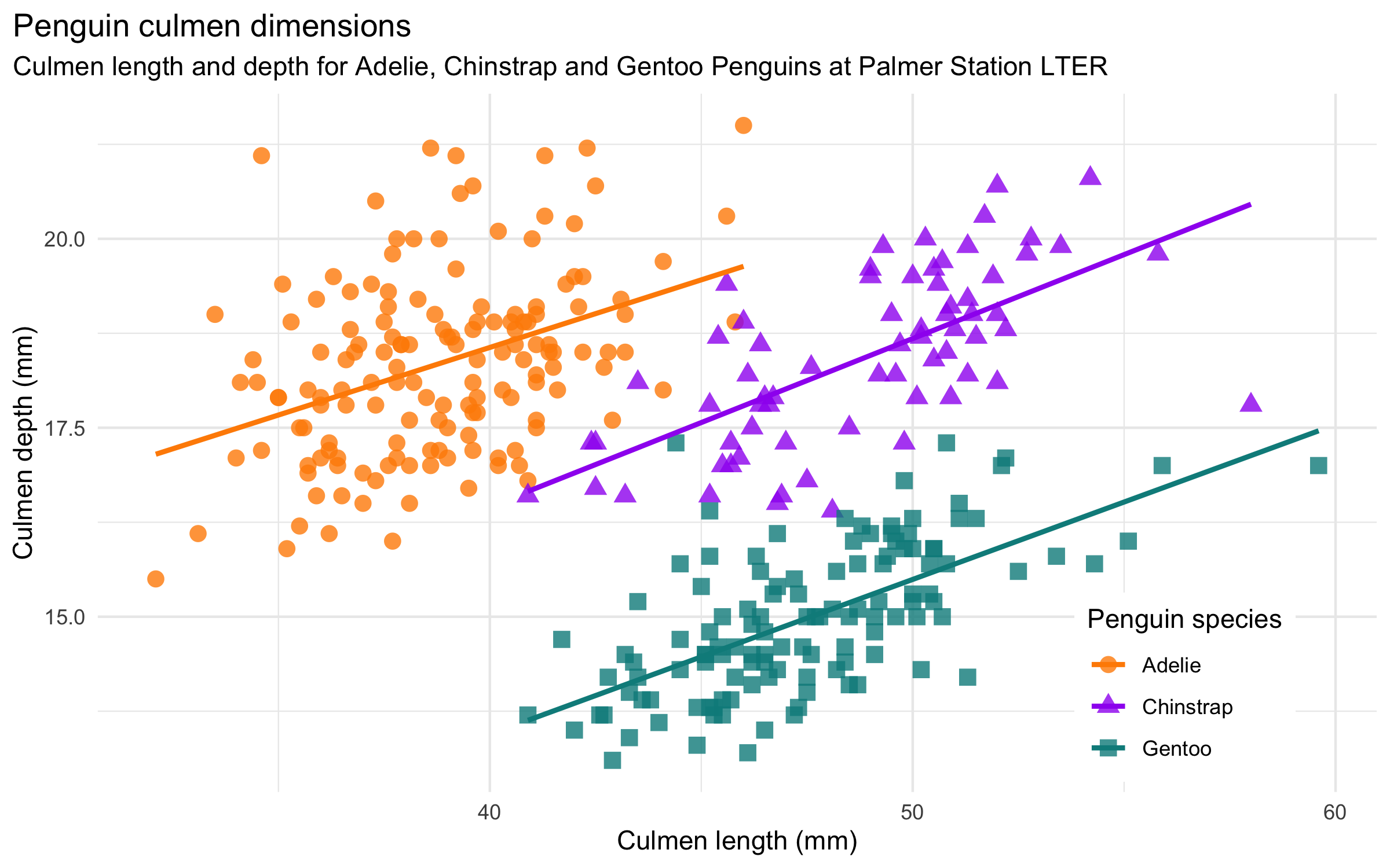
The data is from a published study on Antarctic penguins. It offers great opportunities for regression analysis, cluster analysis, etc. Here are two sample charts from the Github Readme:

Histogram of penguin flipper lengths colored by species


Scatterplot of culmen length and depth clustered by species

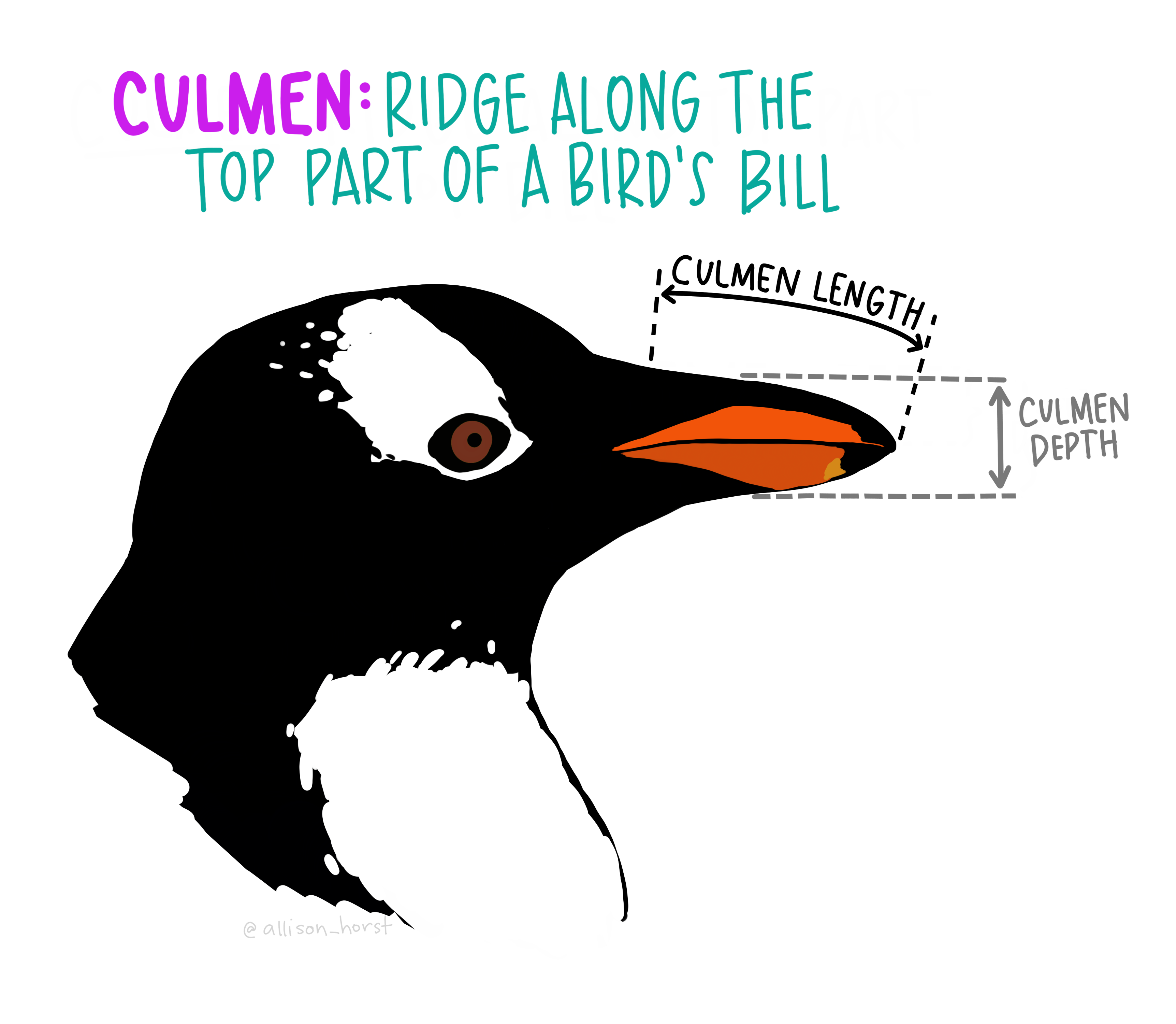
What’s a culmen you may ask? They’ve illustrated that nicely:

Illustration of a penguin culmen

Links and Credits

The data set is available at Github here: https://github.com/allisonhorst/penguins 

A CSV file of the full data set is available in the data-raw sub-directory. Here is a direct link. (You can view the raw version and then save it as a CSV file from your browser.)

Data were collected and made available by Dr. Kristen Gorman and the Palmer Station, Antarctica LTER, a member of the Long Term Ecological Research Network.

The data was used in the published study freely available here:

Gorman KB, Williams TD, Fraser WR (2014) Ecological Sexual Dimorphism and Environmental Variability within a Community of Antarctic Penguins (Genus Pygoscelis). PLoS ONE 9(3): e90081. doi:10.1371/journal.pone.0090081


Tableau Tip: Group Years into Decades Using Calculated Fields

In a recent Tableau project, I wanted to divide a long span of years into decades, as this would provide a more visually effective way to grasp the growth of revenue from top movies (data from The Movie Database) over time. With a little searching, I found the pieces I needed. Below I’ll include a description of my process, followed by links to the helpful sources of insight I found on this topic.

First, here is the visualization with total revenues year by year. Notice that despite its current width you still have to scroll left to reach the early 1900s. Meanwhile, the difference year to year is not in itself that interesting.

Top TMDB movie revenue totals by year a partial view

Now here is the visualization when years are chunked into decades. Much more effective!

Top TMDB movies total revenue by decade

DISCLAIMER: These charts use revenue numbers as entered in The Movie Database by contributors based on publicly reported figures. Thus, the data includes only a portion of all movies. I’ve as yet made no adjustments for inflation.

Getting to Decades from Dates

Now for the process of getting decades from dates. I broke my approach into two steps:

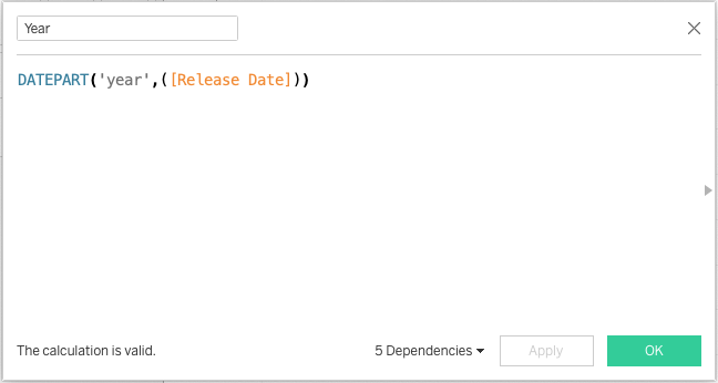
  1. I first created a calculated field to pull the Year from the Release Dates field, using Tableau’s DATEPART function.

    Calculated field to get only the Year from the date information in Release Date

    Once that field was created, I moved the new calculated field from Measures to Dimensions, where it should be.

  2. Then I created a Decades dimension as an additional calculated field. This calculation uses Year and the modulo operator to round each year down to the nearest multiple of 10.

    Calculated field to round each year down to its decade using modulo

    Then, similarly, once created, I made this calculated field a Dimension.
    That’s all it took!

Many thanks to Nick Parsons and Erik Bokobza for their helpful replies in the Tableau Community Forums. Links below.

Recommended Reads

The data revolution is now transforming the world of finance

This article from Tech Republic is worth a read. In summary: The data revolution is now transforming the world of finance. A recent Deloitte survey reveals that traditional roles are being automated. To be a human working in finance, you need skills in data science, analytics, and visualization. More than manipulating spreadsheets, you need to create business value with data-informed innovations.

The finance robots are coming — TechRepublic.com

Balancing Clarity and Creativity in Data Visualization

I’ve been reflecting on Elijah Meeks’ provocative essay, “3rd Wave Data Visualization”. In this post, I want to reflect on the tension between his first and third “waves.” I’ll refer to these as attitudes. (Meeks himself acknowledges that none of his “waves” have washed away. Each lives on.) He refers to them as Wave 1: Clarity and Wave 3: Convergence.

Upon re-reading his argument a few times, I believe we may useful understand the contrast Meeks highlights as the tension between these two imperatives:

Attitude 1: Design with Clarity. (Make sure we don’t miss the message.)

Attitude 2: Bring back the Creativity and Fun. (Give us some enjoyment.)

I’ll talk about these attitudes in more detail in a later post.

For now, I’m going to spend some time going out and evaluating a number of data visualizations bearing in mind questions such as these:

  1. How clear is this visualization? How easy is it to understand and interpret? Is that a good or a bad thing?
  2. How creative and fun is this visualization? Am I motivated to explore it further? Why or why not?
  3. Are there times, places, and audiences for whom clarity is more important than creativity? And vice versa?

The Tableau Public Gallery is a good place to start. And there are many others.

I’d be interested in your responses below. Include a link to a relevant data visualization.

I’ll report back with an update to this post.

Once again, the NY Times demonstrates the value of interactive data visualization

This impressive interactive data visualization demonstrates the value of the format. More than merely interesting, or intriguing, or even fun — it massively amplifies the communicative power of its subject matter.

Check it out:

How to Cut U.S. Emissions Faster? Do What These Countries Are Doing.
By Brad Plumer and Blacki Migliozzi — FEB. 13, 2019

NYTimes_DataViz_Carbon_Reduction_13Feb2019